Transitions and Networks
Different path sampling approaches use different kinds of ensembles. But what they all share in common is that those ensembles represent some network of transitions.
Under most circumstances, the user can directly work with
TransitionNetworks, and never needs to work
directly with Ensembles. This document describes the
internal structure of TransitionsNetworks, and
explains how to customize that structure with different ensembles if so
desired.
This also covers some of the interface between TransitionNetworks and MoveStrategy objects. When developing
new methodologies, this interface allows for high levels of flexibility. A
new TransitionNetwork could be combined with a customized
MoveStrategy to develop all sorts of path-sampling-like
approaches.
Networks are made of Transitions
A transition describes a set of paths with certain allowed initial and final
conditions. There are two groups of transitions that are important when
working with networks. First, there are the
sampling_transitions, which are what are
actually sampled by the dynamics. Then there are
analysis_transitions (or just
transitions) which are the subjects of analysis.
The difference between these is easily described in the context of MSTIS. With MSTIS, you use one set of ensembles to sample the transitions from a given state to all other states. So you would sample \(A\to (B \text{ or } C)\), but the analysis transitions would include separate studies of \(A\to B\) and \(A\to C\).
The network is defined by the combination of what the underlying transitions to study are, and the approach used to study them. It defines a set of path ensembles which are sampled during the dynamics, and the way to combine those afterward into results that connect to physical meaning.
Handcrafting Networks
Beyond the simple tools to customize the networks you study, you can
manually create them with whatever complexity you desire. The
Network level of code is designed to interact
with the MoveScheme and MoveStrategy code, as well as
with some of the analysis tools. As long as
you implement a few items, your custom Network
will work seamlessly with those.
The main point is that there are two aspects of the network: there’s the sampling network, which is organizes the ensembles as used in sampling, and the analysis network, which actually consists of the specific transitions you’re interested in studying.
Handcrafting the sampling network
The sampling network consists of three objects:
network._sampling_transitions: a list of transitions; contains all the normal ensembles (accessible asnetwork.sampling_transitions)network.special_ensembles: a dictionary with strings for keys, describing the type of ensemble, and dictionaries for values. Those value dictionaries have the ensembles themselves as keys, and a list of associated transitions as values.network.hidden_ensembles: this list is empty when built by the network, and is set by the MoveScheme if necessary. This consists of ensembles that aren’t part of the network, but are part of the move scheme.
The special ensembles need to have the correct key names to work with the
MoveScheme and MoveStrategy subsystem. These are
'minus' for the minus interfaces, and 'ms_outer' for the multiple
state outer interfaces.
If you do that, then MoveStrategy and MoveScheme will
work with your networks.
Handcrafting the analysis network
The analysis network is determined by the list of all state pairs that
represent the transitions you’re studying. It is contained in the
network.transitions dictionary,
which has keys of tuples in the form (stateA, stateB) with values of the
Transition object that describes the \(A\to B\) transition.
During analysis calculations, you will often perform the analysis on the
sampling network, but copy the results of that analysis to the transition
network using
analysis_transition.copy_analysis_from(sampling_transition). For example, in MSTIS, you only run one
crossing probability analysis per state (per sampling transition), but this
is used to link to all the specific state-to-state transitions in the
analysis network.
Examples of Networks and Transitions
Two-state network
It is perhaps easiest to understand the idea of networks and transitions if we visualize them for the case of transition interface sampling. Let’s take one of the commonly-used illustrations of TIS as a starting point:
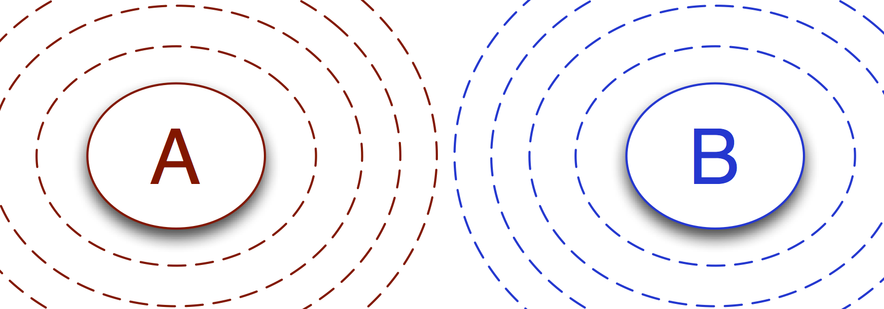
Here we see two transitions: \(A\to B\) and \(B\to A\). In this
simple example, there is no distinction between sampling transitions and
analysis transitions. Each transition consists of several ensembles. The
ensembles define the paths that will actually be sampled during the path
sampling simulation. The transitions provide a context for analyzing those
results: in TIS, we combine results from sampling multiple ensembles in a
specific way in order to determine rates. The Transition object
keeps the information on how to combine information from its various
ensembles.
In practice, this network can be created as either an MSTISNetwork
or a MISTISNetwork:
# mstis version
mstis = paths.MSTISNetwork([
    (stateA, interfacesAB, orderparameterAB),
    (stateB, interfacesBA, orderparameterBA)
])

# mistis version
mistis = paths.MISTISNetwork([
    (stateA, interfacesAB, orderparameterAB, stateB),
    (stateB, interfacesBA, orderparameterBA, stateA)
])
Both of these would give the same behavior.
Note that there are other approaches that could give different networks. By
default, both MSTISNetwork and MISTISNetwork create a
“multiple state outer interface,” which links the two transitions. Whether
this interface is actually used depends on the MoveScheme:
however, another network type might not even make it. Similarly, the
transitions in both of these create a MinusInterfaceEnsemble,
which could be removed.
For simplicity, we recommend that users who wish to avoid making use of
these ensembles adjust the MoveStrategy and MoveScheme
to manage that, rather than creating a new TransitionNetwork.
Three-state networks
Now let’s consider a 3-state system. In the image below, we illustrate the
sampling network for an MSTISNetwork for a 3-state system.
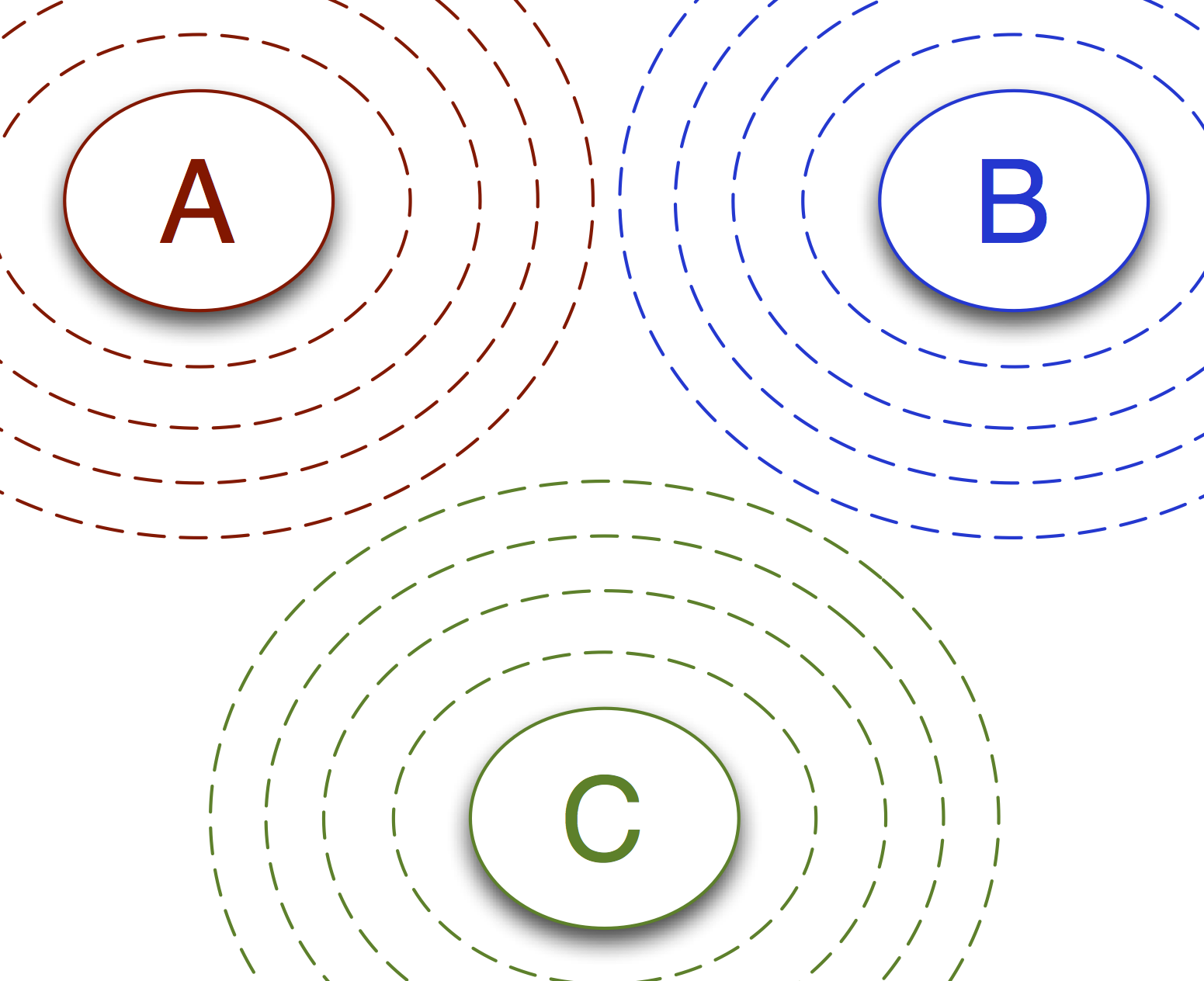
In this example, there are 3 sampling transitions:
- from state A, through the interfaces associated with A, and to either state B or state C
- from state B, through the interfaces associated with B, and to either state A or state C
- from state C, through the interfaces associated with C, and to either state A or state B
However, there are 6 analysis transitions: \(A\to B\), \(A\to C\), \(B\to A\), \(B\to C\), \(C\to A\), and \(C\to B\). Each sampling transition samples for two analysis transitions.
When you want a rate, you want the rate for the analysis transition. For example, you would typically want a rate for the \(A\to B\) process, not the \(A\to (B \text{ or } C)\) process, which is what the sampling transition would give you. However, the sampling transitions can be much more efficient to sampling: the number of analysis transitions scales as the square of the number of states, while, in MSTIS, the number of sampling transitions scales linearly with (actually, is equal to) the number of states.
MISTISNetworks, on the other hand, have a sampling
transition for each analysis transition. This can give the advantage of
allowing a better order parameter to be used as an approximation to very
different reaction coordinates coming from the same state. It also allows
you to focus on only a subset of the \(N^2\) possible transitions.
By distinguishing between sampling transitions and analysis transitions, OpenPathSampling makes it easy to allow this kind of flexibility in the underlying sampling style, while still making it very easy to set up a given kind of network with minimal code.