Obtaining the first trajectories for a Toy Model

Tasks covered in this notebook:

• Setting up a system using the OPS toy engine

• Using a user-defined function to create a collective variable

• Using collective variables to define states and interfaces

• Storing things manually

Path sampling methods require that the user supply an input path for each path ensemble. This means that you must somehow generate a first input path. The first rare path can come from any number of sources. The main idea is that any trajectory that is nearly physical is good enough. This is discussed more in the OPS documentation on initial trajectories.

In this example, we use a bootstrapping/ratcheting approach, which does create paths satisfying the true dynamics of the system. This approach is nice because it is quick and convenient, although it is best for smaller systems with less complicated transitions. It works by running normal MD to generate a path that satisfies the innermost interface, and then performing shooting moves in that interface’s path ensemble until we have a path that crosses the next interface. Then we switch to the path ensemble for the next interface, and shoot until the path crossing the interface after that. The process continues until we have paths for all interfaces.

In this example, we perform multiple state (MS) TIS. Therefore we do one bootstrapping calculation per initial state.

# Basic imports
from __future__ import print_function
import openpathsampling as paths
import numpy as np
%matplotlib inline

# used for visualization of the 2D toy system
# we use the %run magic because this isn't in a package
%run ../resources/toy_plot_helpers.py

Basic system setup

First we set up our system: for the toy dynamics, this involves defining a potential energy surface (PES), setting up an integrator, and giving the simulation an initial configuration. In real MD systems, the PES is handled by the combination of a topology (generated from, e.g., a PDB file) and a force field definition, and the initial configuration would come from a file instead of being described by hand.

# convenience for the toy dynamics
import openpathsampling.engines.toy as toys

Set up the toy system

For the toy model, we need to give a snapshot as a template, as well as a potential energy surface. The template snapshot also includes a pointer to the topology information (which is relatively simple for the toy systems.)

# Toy_PES supports adding/subtracting various PESs.
# The OuterWalls PES type gives an x^6+y^6 boundary to the system.
pes = (
    toys.OuterWalls([1.0, 1.0], [0.0, 0.0])
    + toys.Gaussian(-0.7, [12.0, 12.0], [0.0, 0.4])
    + toys.Gaussian(-0.7, [12.0, 12.0], [-0.5, -0.5])
    + toys.Gaussian(-0.7, [12.0, 12.0], [0.5, -0.5])
)

topology=toys.Topology(
    n_spatial=2,
    masses=[1.0, 1.0],
    pes=pes
)

Set up the engine

The engine needs the template snapshot we set up above, as well as an integrator and a few other options. We name the engine; this makes it easier to reload it in the future.

integ = toys.LangevinBAOABIntegrator(dt=0.02, temperature=0.1, gamma=2.5)

options={
    'integ': integ,
    'n_frames_max': 5000,
    'n_steps_per_frame': 1
}

toy_eng = toys.Engine(
    options=options,
    topology=topology
).named('toy_engine')

template = toys.Snapshot(
    coordinates=np.array([[-0.5, -0.5]]),
    velocities=np.array([[0.0,0.0]]),
    engine=toy_eng
)

toy_eng.current_snapshot = template

Finally, we make this engine into the default engine for any PathMover that requires an one (e.g., shooting movers, minus movers).

paths.PathMover.engine = toy_eng

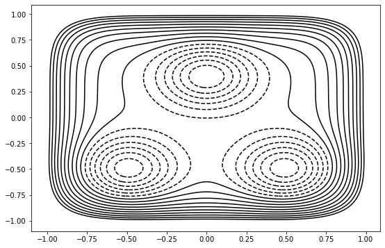
Now let’s look at the potential energy surface we’ve created:

plot = ToyPlot()
plot.contour_range = np.arange(-1.5, 1.0, 0.1)
plot.add_pes(pes)
fig = plot.plot()

Defining states and interfaces

TIS methods usually require that you define states and interfaces before starting the simulation. State and interfaces are both defined in terms of Volume objects. The most common type of Volume is one based on some set of collective variables, so the first thing we have to do is to define the collective variable.

For this system, we’ll define the collective variables as circles centered on the middle of the state. OPS allows us to define one function for the circle, which is parameterized by different centers. Note that each collective variable is in fact a separate function.

def circle(snapshot, center):
    import math
    return math.sqrt((snapshot.xyz[0][0]-center[0])**2
                     + (snapshot.xyz[0][1]-center[1])**2)

opA = paths.CoordinateFunctionCV(name="opA", f=circle, center=[-0.5, -0.5])
opB = paths.CoordinateFunctionCV(name="opB", f=circle, center=[0.5, -0.5])
opC = paths.CoordinateFunctionCV(name="opC", f=circle, center=[0.0, 0.4])

Now we define the states and interfaces in terms of these order parameters. The CVRangeVolumeSet gives a shortcut to create several volume objects using the same collective variable.

stateA = paths.CVDefinedVolume(opA, 0.0, 0.2)
stateB = paths.CVDefinedVolume(opB, 0.0, 0.2)
stateC = paths.CVDefinedVolume(opC, 0.0, 0.2)

interfacesA = paths.VolumeInterfaceSet(opA, 0.0, [0.2, 0.3, 0.4])
interfacesB = paths.VolumeInterfaceSet(opB, 0.0, [0.2, 0.3, 0.4])
interfacesC = paths.VolumeInterfaceSet(opC, 0.0, [0.2, 0.3, 0.4])

Build the MSTIS transition network

Once we have the collective variables, states, and interfaces defined, we can create the entire transition network. In this one small piece of code, we create all the path ensembles needed for the simulation, organized into structures to assist with later analysis.

ms_outers = paths.MSOuterTISInterface.from_lambdas(
    {ifaces: 0.5
     for ifaces in [interfacesA, interfacesB, interfacesC]}
)
mstis = paths.MSTISNetwork(
    [(stateA, interfacesA),
     (stateB, interfacesB),
     (stateC, interfacesC)],
    ms_outers=ms_outers
)

Bootstrap to fill all interfaces

Now we actually run the bootstrapping calculation. The full_bootstrap function requires an initial snapshot in the state, and then it will generate trajectories satisfying TIS ensemble for the given interfaces. To fill all the ensembles in the MSTIS network, we need to do this once for each initial state.

initA = toys.Snapshot(
    coordinates=np.array([[-0.5, -0.5]]),
    velocities=np.array([[1.0,0.0]]),
)
bootstrapA = paths.FullBootstrapping(
    transition=mstis.from_state[stateA],
    snapshot=initA,
    engine=toy_eng,
    forbidden_states=[stateB, stateC],
    extra_interfaces=[ms_outers.volume_for_interface_set(interfacesA)]
)
gsA = bootstrapA.run()

DONE! Completed Bootstrapping cycle step 49 in ensemble 4/4.

initB = toys.Snapshot(
    coordinates=np.array([[0.5, -0.5]]),
    velocities=np.array([[-1.0,0.0]]),
)

bootstrapB = paths.FullBootstrapping(
    transition=mstis.from_state[stateB],
    snapshot=initB,
    engine=toy_eng,
    forbidden_states=[stateA, stateC]
)
gsB = bootstrapB.run()

DONE! Completed Bootstrapping cycle step 56 in ensemble 3/3.

initC = toys.Snapshot(
    coordinates=np.array([[0.0, 0.4]]),
    velocities=np.array([[0.0,-0.5]]),
)
bootstrapC = paths.FullBootstrapping(
    transition=mstis.from_state[stateC],
    snapshot=initC,
    engine=toy_eng,
    forbidden_states=[stateA, stateB]
)
gsC = bootstrapC.run()

DONE! Completed Bootstrapping cycle step 29 in ensemble 3/3.

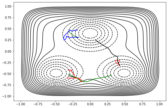
Now that we’ve done that for all 3 states, let’s look at the trajectories we generated.

plot.plot([s.trajectory for s in gsA]+[s.trajectory for s in gsB]+[s.trajectory for s in gsC]);

Finally, we join these into one SampleSet. The function relabel_replicas_per_ensemble ensures that the trajectory associated with each ensemble has a unique replica ID.

total_sample_set = paths.SampleSet.relabel_replicas_per_ensemble(
    [gsA, gsB, gsC]
)

Storing stuff

Up to this point, we haven’t stored anything in files. In other notebooks, a lot of the storage is done automatically. Here we’ll show you how to store a few things manually. Instead of storing the entire bootstrapping history, we’ll only store the final trajectories we get out.

First we create a file. When we create it, the file also requires the template snapshot.

storage = paths.Storage("mstis_bootstrap.nc", "w")

The storage will recursively store data, so storing total_sample_set leads to automatic storage of all the Sample objects in that sampleset, which in turn leads to storage of all the ensemble, trajectories, and snapshots.

Since the path movers used in bootstrapping and the engine are not required for the sampleset, they would not be stored. We explicitly store the engine for later use, but we won’t need the path movers, so we don’t try to store them.

storage.save(total_sample_set)
storage.save(toy_eng)

(store.engines[DynamicsEngine] : 1 object(s),
 10,
 312146789929318672826458068150699163670)

Now we can check to make sure that we actually have stored the objects that we claimed to store. There should be 0 pathmovers, 1 engine, 12 samples (4 samples from each of 3 transitions), and 1 sampleset. There will be some larger number of snapshots. There will also be a larger number of ensembles, because each ensemble is defined in terms of subensembles, each of which gets saved.

print("PathMovers:", len(storage.pathmovers))
print("Engines:", len(storage.engines))
print("Samples:", len(storage.samples))
print("SampleSets:", len(storage.samplesets))
print("Snapshots:", len(storage.snapshots))
print("Ensembles:", len(storage.ensembles))
print("CollectiveVariables:", len(storage.cvs))

PathMovers: 0
Engines: 1
Samples: 10
SampleSets: 1
Snapshots: 732
Ensembles: 120
CollectiveVariables: 6

Finally, we close the storage. Not strictly necessary, but a good habit.

storage.close()